As mentioned before, we will be using the data from this study by Santos & Duarte (2016). If you want to run the code below on your local machine, please follow the links in their PeerJ article to download their data from FigShare. Alternatively, if you just want to follow along with the code, you can see all of the code, outputs, and figures below without having to download any data.
If you do download the data, please save it in this structure:
YOUR_FOLDER_HERE/               # Name of the project folder on your local computer
└── data/                       # data subfolder
    └── BDS/
        ├── trials/              # These are the individual trials data files downloaded from Figshare
            └── BDS00001.csv         # 60s of stabilometer data for trial 1
            └── ...
            └── BDS01956.csv         # 60s of stabilometer data for trial 1956
        └── output/             # This is where we will store outputs generated by the code
        └── BDSinfo.csv         # This is the demographic datafile from FigShare. This file maps trials to subjects.
        # Note that on figshare, the BDSinfo.csv is in the same folder as the individual trial data
        # we move it out of that folder to make some of our automated steps easier.
Note that our data differ from the original Santos & Duarte (2016) dataset. The original data were collected and processed to a very high standard to maximize their utility for biomechanics researchers. Because we want to use these data for teaching purposes, we manipulated some of the original data to introduce artifacts and other types of errors that we want to catch in our pipeline. Thus, the data presented below are for teaching purposes only and we explicitly do not make the “doctored” data available to avoid confusion with the original dataset. If readers are interested in following along step by step, they should download the original data from their source, but remember that those data will not include the errors we built in for teaching purposes.
In the code chunks below, you can toggle between the R and Python implementations. We have tried to keep the code as similar as possible between the two languages, but it is important to remember that:
There is never only one way to things in programming, although some ways are better than others (and we try to show only “good” ways).
Each programming language is different. So, even though we try to keep the code as structurally similar as possible, there often won’t be a one-to-one translation between languages.
In the chunks below, we show the structure of the “raw” data after they have been merged into one master data files (rather than individual .csv files for every subject on every trial).
The first few columns track structural information about how these data are organized:
Trial - the trial number which was used to index the original raw data files.
Subject - the unique subject identification number, each subject has ~4 trials and ~60s worth of data per trial.
Vision - was the trial completed with eyes open or eyes closed.
Surface - was the trial completed on a firm surface or a foam surface.
Time - time, in seconds, within each trial. Trials were, in general, 60s long.
… and the last few columns are the key dependent variables tracked continuously throughout each trial:
Fx, Fy, and Fz - force in each plane of the force plate.
Mx, My, and Mz - moment arms corresponding to the forces in each plane.
CoPx and CoPy - the center of pressure as a point, in the x- and y-planes of force plate, calculated from the preceding forces and moment arms.
2 Quality Assurance & Feature Extraction
From raw Center of Pressure (COP) time-series data \((COP_x, COP_y)\), we will calculate key biomechanical variables that a researcher might be interested in:
Path Lengths: Sum of absolute step distances across axes: \[\text{PathLength}_{\text{AP}} = \sum_{n=1}^{N-1} |COP_{y, n+1} - COP_{y, n}|\]\[\text{PathLength}_{\text{Total}} = \sum_{n=1}^{N-1} \sqrt{(COP_{x, n+1} - COP_{x, n})^2 + (COP_{y, n+1} - COP_{y, n})^2}\]
95% Confidence Ellipse Area & Boundary: \[\text{Area}_{95} = 2 \pi F_{0.95, 2, N-2} \sqrt{\lambda_1 \lambda_2}\] where \(\lambda_1, \lambda_2\) are eigenvalues of the \((COP_x, COP_y)\) covariance matrix.
Mean Velocity: The average of the change in center of pressure in anterior-posterior (AP) and medial-lateral (ML) axes separately.
Before visualizing these features, we also flag a few common structural and signal-level problems that occur in this kind of research. Each flag targets a different stage where something can go wrong:
flag_sample_count – does this trial have roughly the expected number of samples? Trials were meant to run 60s at 100Hz (6,000 samples), so we compare each trial’s row count to the modal count across all trials and flag anything off by more than 10 samples. This is a completeness check: did the recording actually capture the full trial, or did it start late, end early, or get truncated when the file was written to disk?
flag_time_gap – within a trial, does Time advance smoothly at the expected ~0.01s interval, with no backward jumps or repeats? This is a temporal integrity check: it catches dropped samples or corrupted timestamps. This matters more than it might seem, because path-length and velocity are both computed from consecutive-sample differences – a silent gap in time doesn’t just look wrong, it quietly inflates those estimates without ever producing an obviously “broken” value.
flag_fz_unweighting – does the vertical force (Fz) ever drop well below what’s typical for that trial? Fz roughly tracks how much of the participant’s body weight is loading the plate, so a sustained drop below 70% of the trial’s median suggests the participant wasn’t fully weight-bearing for part of the trial – a partial step off, a hand momentarily on a rail, or (especially relevant in older or clinical populations) a spotter briefly providing support. Unlike the first two flags, this one isn’t about the recording – it’s about whether the trial was performed the way the protocol intended.
We combine these into a single flag_any column so we have one place to filter for problem trials.
Errors like these are common in this kind of research simply because of scale: a large postural-sway study generates many independently-recorded, largely unattended trials – here, 163 participants x 12 trials each – and at that volume, rare per-trial failure rates become guaranteed somewhere in the dataset. Hardware and software issues (a force plate briefly losing connection, a buffer overflow, a file that didn’t finish writing) and participant/protocol issues (stepping off the plate, needing brief physical support) are each individually uncommon but collectively inevitable across thousands of trials – which is exactly why we build automated checks into the pipeline rather than relying on a raw export being clean.
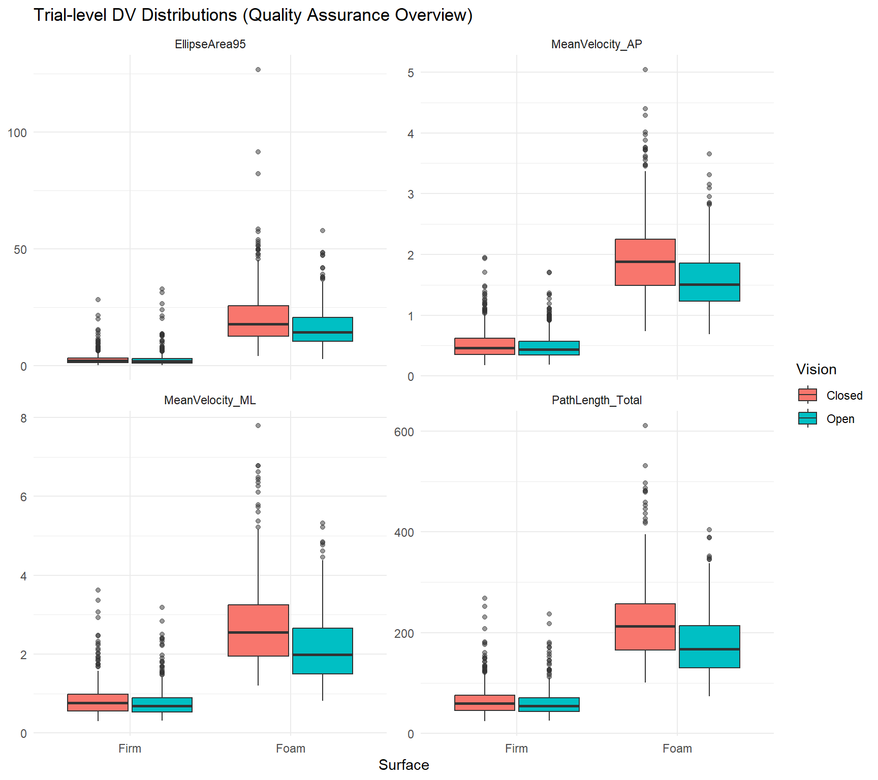
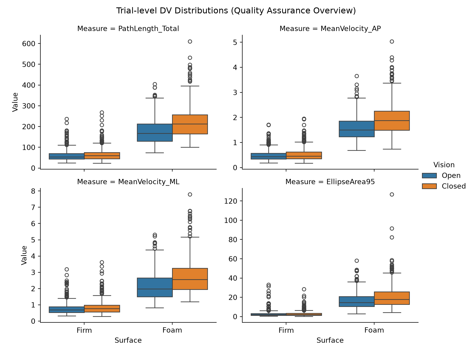
In the plots below, we show how we can visualize “trial-level” data, calculated across all 60s in each trial, in each condition. This is a high-level summary plot that allows you to visualize data from many different participants at once. This kind of plot would be useful identifying influential participants who do not fit general patterns and may even be considered “outliers”. For instance, only one participant has a total path length over 600 in the eyes closed/foam surface condition. It would be worth checking notes from the data collection to see if there was an anomaly in the testing that might explain why this person is a statistical outlier. Broadly, we do not recommend removing outliers for statistical reasons alone (e.g., there will always be an extreme 1%, so we cannot remove it for its extreme-ness alone), but identifying statistical outliers is often a useful first step in ensuring data quality.
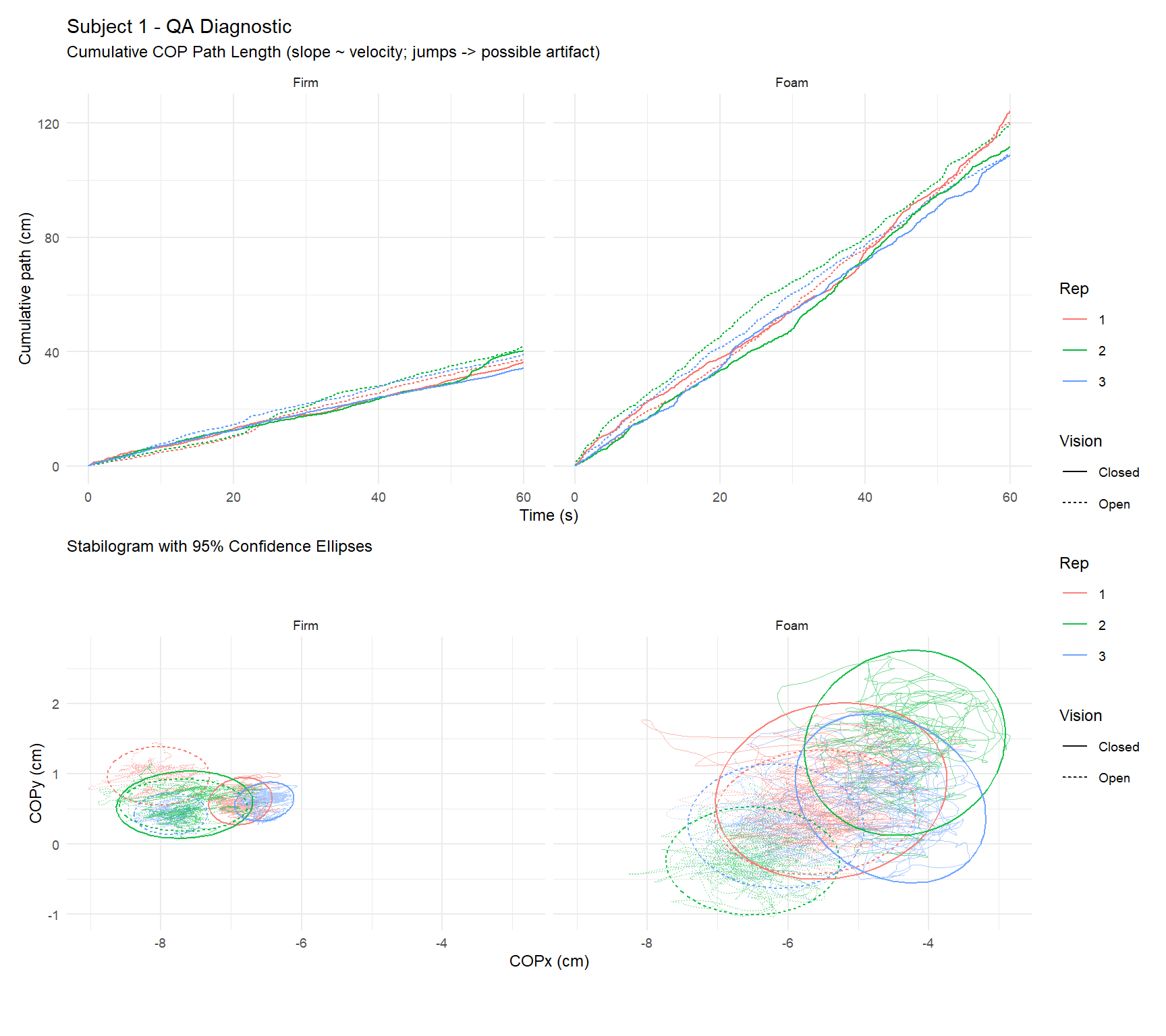
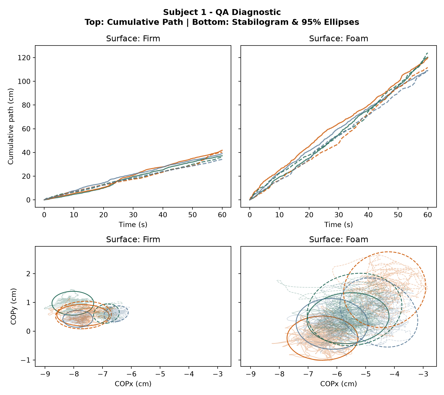
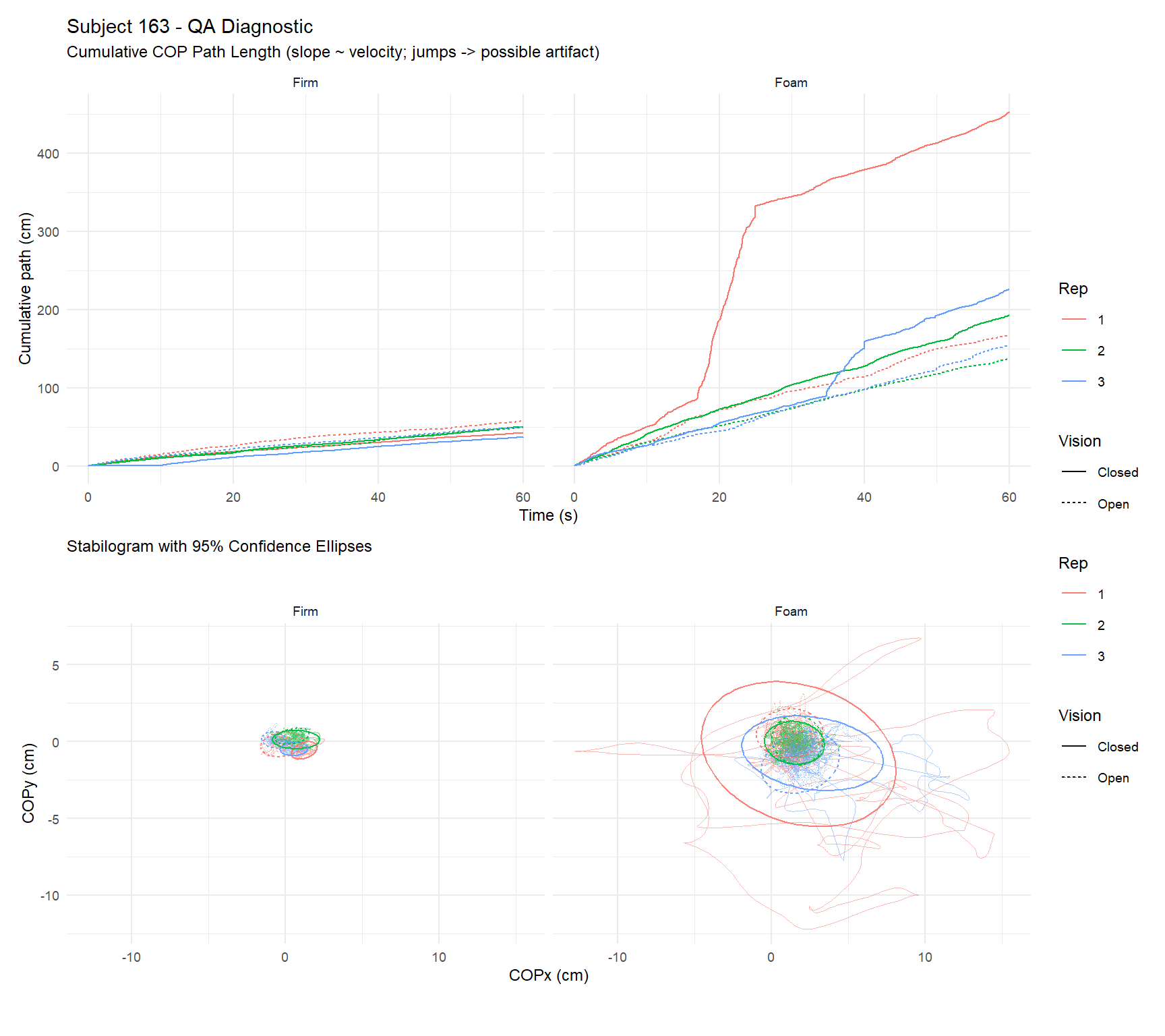
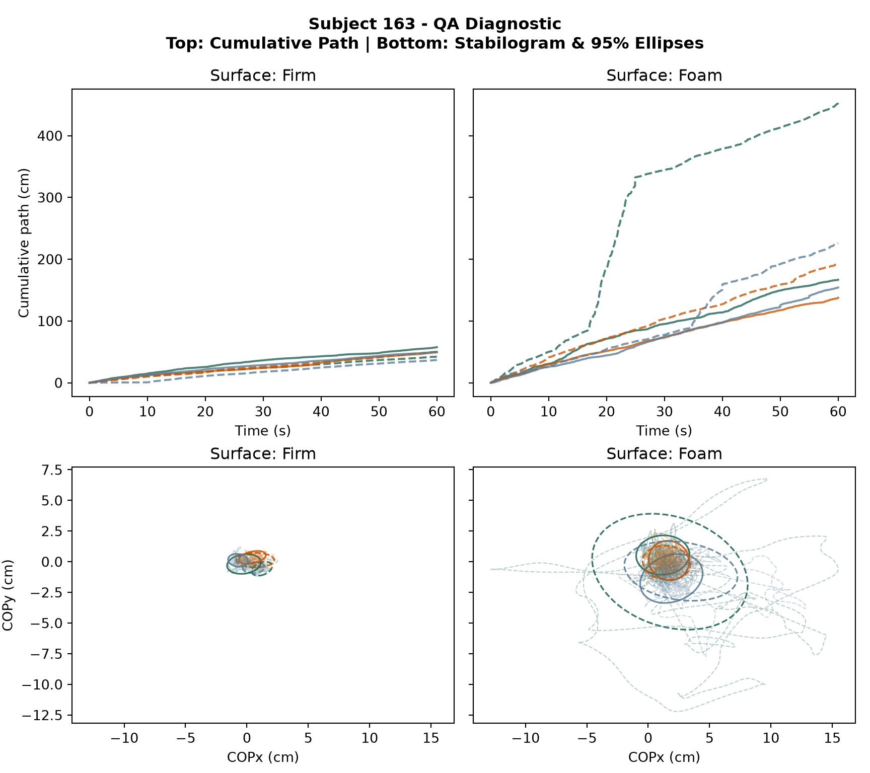
Next, we show a quality assurance graphic that we might make for a single subject. This graphic shows what is happening on a “trial-level” within a given subject, e.g., cumulative path length for the CoP and two dimensional area of CoP dispersion over time.
Rather than rebuilding this augmented dataset and re-looping over all 163 subjects twice (once to illustrate a “clean” subject, once to illustrate a subject with built-in errors), we do the expensive part once, in a single prep step below. That step (1) builds master_aug and the per-trial Rep indicator, (2) splits the data by subject once instead of re-filtering the full ~11-million-row table on every subject, and (3) writes one diagnostic PNG per subject to disk – but only for subjects whose PNG doesn’t already exist.
Keep in mind we started with over 11 million rows of data! There is no way a human operator can do meaningfully do quality assurance by hand when data sets get that large. However, if we build up our skills with data visualization, we can turn millions of rows and columns of data into a few meaningful graphics.
Source Code
---title: "Data Import & Quality Assurance"subtitle: "A Parallel Guide in R and Python"---# Import and Merge DataAs mentioned before, we will be using the data from this study by [Santos & Duarte (2016)](https://peerj.com/articles/2648/). If you want to run the code below on your local machine, please follow the links in their PeerJ article to download their data from FigShare. Alternatively, if you just want to follow along with the code, you can see all of the code, outputs, and figures below without having to download any data. If you do download the data, please save it in this structure:```textYOUR_FOLDER_HERE/ # Name of the project folder on your local computer└── data/ # data subfolder └── BDS/ ├── trials/ # These are the individual trials data files downloaded from Figshare └── BDS00001.csv # 60s of stabilometer data for trial 1 └── ... └── BDS01956.csv # 60s of stabilometer data for trial 1956 └── output/ # This is where we will store outputs generated by the code └── BDSinfo.csv # This is the demographic datafile from FigShare. This file maps trials to subjects. # Note that on figshare, the BDSinfo.csv is in the same folder as the individual trial data # we move it out of that folder to make some of our automated steps easier.```**Note that our data differ from the original Santos & Duarte (2016) dataset.** The original data were collected and processed to a very high standard to maximize their utility for biomechanics researchers. Because we want to use these data for teaching purposes, we manipulated some of the original data to introduce artifacts and other types of errors that we want to catch in our pipeline. Thus, the data presented below are for teaching purposes only and we explicitly do not make the "doctored" data available to avoid confusion with the original dataset. If readers are interested in following along step by step, they should download the original data from their source, but remember that those data will not include the errors we built in for teaching purposes.In the code chunks below, you can toggle between the `R` and `Python` implementations. We have tried to keep the code as similar as possible between the two languages, but it is important to remember that:1. There is never only one way to things in programming, although some ways are better than others (and we try to show only "good" ways).2. Each programming language is different. So, even though we try to keep the code as structurally similar as possible, there often won't be a one-to-one translation between languages. In the chunks below, we show the structure of the "raw" data after they have been merged into one master data files (rather than individual .csv files for every subject on every trial). ::: panel-tabset## R (`tidyverse` & `data.table`)```{r}#| label: script00-rlibrary(reticulate)library(tidyverse)library(data.table)library(arrow)# 1. Read metadatainfo_path <-"./data/BDS/BDSinfo.txt"info_raw <-read_tsv(info_path, show_col_types =FALSE)info <- info_raw %>%select(Trial, Subject, Vision, Surface, Age, AgeGroup, Gender, Height, Weight, BMI) %>%mutate(Subject =as.integer(Subject),Vision =factor(Vision, levels =c("Open", "Closed")),Surface =factor(Surface, levels =c("Firm", "Foam")),AgeGroup =factor(AgeGroup),Gender =factor(Gender) )# 2. Batch-read raw trial filestrial_files <-list.files("./data/BDS/trials", pattern ="^BDS\\d+\\.txt$", full.names =TRUE)trial_ids <- tools::file_path_sans_ext(basename(trial_files))read_one_trial <-function(path, trial_id) {fread(path, header =TRUE, sep ="\t", showProgress =FALSE) %>%as_tibble() %>%rename_with(~str_trim(str_remove(.x, "\\[.*\\]"))) %>%mutate(Trial = trial_id, .before =1)}trial_list <-map2(trial_files, trial_ids, read_one_trial)all_trials <-bind_rows(trial_list)# 3. Merge & Savemaster <- all_trials %>%left_join(info, by ="Trial") %>%relocate(Trial, Subject, Vision, Surface, Age, AgeGroup, Gender, Height, Weight, BMI, .before = Time)dir.create("./data/BDS/output", recursive =TRUE, showWarnings =FALSE)arrow::write_parquet(master, "./data/BDS/output/BDS_master.parquet")glimpse(master)```## Python (`pandas` & `pyarrow`)```{python}#| label: script00-pythonimport sysimport globimport osimport pandas as pd# 1. Read metadatainfo_raw = pd.read_csv("./data/BDS/BDSinfo.txt", sep="\t")cols = ["Trial", "Subject", "Vision", "Surface", "Age", "AgeGroup", "Gender", "Height", "Weight", "BMI"]info = info_raw[cols].copy()info["Subject"] = info["Subject"].astype(int)info["Vision"] = pd.Categorical(info["Vision"], categories=["Open", "Closed"])info["Surface"] = pd.Categorical(info["Surface"], categories=["Firm", "Foam"])# 2. Batch-read raw trial filestrial_files =sorted(glob.glob("./data/BDS/trials/BDS*.txt"))def read_one_trial(path): trial_id = os.path.splitext(os.path.basename(path))[0] df = pd.read_csv(path, sep="\t")# Clean headers (strip units like [cm], [N]) df.columns = df.columns.str.replace(r"\[.*\]", "", regex=True).str.strip() df.insert(0, "Trial", trial_id)return dftrial_list = [read_one_trial(f) for f in trial_files]all_trials = pd.concat(trial_list, ignore_index=True)# 3. Merge & Savemaster = pd.merge(all_trials, info, on="Trial", how="left")os.makedirs("./data/BDS/output", exist_ok=True)master.to_parquet("./data/BDS/output/BDS_master.parquet")master.info()```:::The first few columns track **structural** information about how these data are organized:* `Trial` - the trial number which was used to index the original raw data files.* `Subject` - the unique subject identification number, each subject has ~4 trials and ~60s worth of data per trial.* `Vision` - was the trial completed with eyes open or eyes closed.* `Surface` - was the trial completed on a firm surface or a foam surface.* `Time` - time, in seconds, within each trial. Trials were, in general, 60s long. ... and the last few columns are the key dependent variables tracked continuously throughout each trial:* `Fx`, `Fy`, and `Fz` - force in each plane of the force plate. * `Mx`, `My`, and `Mz` - moment arms corresponding to the forces in each plane.* `CoPx` and `CoPy` - the center of pressure as a point, in the x- and y-planes of force plate, calculated from the preceding forces and moment arms. ------------------------------------------------------------------------# Quality Assurance & Feature ExtractionFrom raw Center of Pressure (COP) time-series data $(COP_x, COP_y)$, we will calculate key biomechanical variables that a researcher might be interested in:1. **Path Lengths**: Sum of absolute step distances across axes: $$\text{PathLength}_{\text{AP}} = \sum_{n=1}^{N-1} |COP_{y, n+1} - COP_{y, n}|$$ $$\text{PathLength}_{\text{Total}} = \sum_{n=1}^{N-1} \sqrt{(COP_{x, n+1} - COP_{x, n})^2 + (COP_{y, n+1} - COP_{y, n})^2}$$2. **95% Confidence Ellipse Area & Boundary**: $$\text{Area}_{95} = 2 \pi F_{0.95, 2, N-2} \sqrt{\lambda_1 \lambda_2}$$ where $\lambda_1, \lambda_2$ are eigenvalues of the $(COP_x, COP_y)$ covariance matrix.3. **Mean Velocity**: The average of the change in center of pressure in anterior-posterior (AP) and medial-lateral (ML) axes separately. Before visualizing these features, we also flag a few common structural and signal-level problems that occur in this kind of research. Each flag targets a different stage where something can go wrong:* **`flag_sample_count`** -- does this trial have roughly the expected number of samples? Trials were meant to run 60s at 100Hz (6,000 samples), so we compare each trial's row count to the *modal* count across all trials and flag anything off by more than 10 samples. This is a **completeness** check: did the recording actually capture the full trial, or did it start late, end early, or get truncated when the file was written to disk?* **`flag_time_gap`** -- within a trial, does `Time` advance smoothly at the expected ~0.01s interval, with no backward jumps or repeats? This is a **temporal integrity** check: it catches dropped samples or corrupted timestamps. This matters more than it might seem, because path-length and velocity are both computed from *consecutive-sample differences* -- a silent gap in time doesn't just look wrong, it quietly inflates those estimates without ever producing an obviously "broken" value.* **`flag_fz_unweighting`** -- does the vertical force (`Fz`) ever drop well below what's typical for that trial? `Fz` roughly tracks how much of the participant's body weight is loading the plate, so a sustained drop below 70% of the trial's median suggests the participant wasn't fully weight-bearing for part of the trial -- a partial step off, a hand momentarily on a rail, or (especially relevant in older or clinical populations) a spotter briefly providing support. Unlike the first two flags, this one isn't about the *recording* -- it's about whether the trial was *performed* the way the protocol intended.We combine these into a single `flag_any` column so we have one place to filter for problem trials.Errors like these are common in this kind of research simply because of scale: a large postural-sway study generates many independently-recorded, largely unattended trials -- here, 163 participants x 12 trials each -- and at that volume, rare per-trial failure rates become *guaranteed* somewhere in the dataset. Hardware and software issues (a force plate briefly losing connection, a buffer overflow, a file that didn't finish writing) and participant/protocol issues (stepping off the plate, needing brief physical support) are each individually uncommon but collectively inevitable across thousands of trials -- which is exactly why we build automated checks into the pipeline rather than relying on a raw export being clean.In the plots below, we show how we can visualize "trial-level" data, calculated across all 60s in each trial, in each condition. This is a high-level summary plot that allows you to visualize data from many different participants at once. This kind of plot would be useful identifying influential participants who do not fit general patterns and may even be considered "outliers". For instance, only one participant has a total path length over 600 in the eyes closed/foam surface condition. It would be worth checking notes from the data collection to see if there was an anomaly in the testing that might explain why this person is a statistical outlier. Broadly, we do not recommend removing outliers for statistical reasons alone (e.g., there will always be an extreme 1%, so we cannot remove it for its extreme-ness alone), but identifying statistical outliers is often a useful first step in ensuring data quality.::: {.panel-tabset}## R (`tidyverse` & `patchwork`)```{r}#| label: script01-r#| fig-width: 9#| fig-height: 8library(tidyverse)library(arrow)library(patchwork)master <- arrow::read_parquet("./data/BDS/output/BDS_master.parquet")# 1. Feature Extraction & Ellipse Mathcompute_path_metrics <-function(x, y, duration_s) { dx <-diff(x) dy <-diff(y) pl_ml <-sum(abs(dx)) pl_ap <-sum(abs(dy)) pl_total <-sum(sqrt(dx^2+ dy^2))tibble(PathLength_AP = pl_ap,PathLength_ML = pl_ml,PathLength_Total = pl_total,MeanVelocity_AP = pl_ap / duration_s,MeanVelocity_ML = pl_ml / duration_s )}compute_ellipse95 <-function(x, y) { n <-length(x) cov_mat <- stats::cov(cbind(x, y)) eig <-eigen(cov_mat) Fval <- stats::qf(0.95, df1 =2, df2 = n -2) area <-2* pi * Fval *sqrt(eig$values[1] * eig$values[2])list(area = area, eig = eig, Fval = Fval, center =c(mean(x), mean(y)))}ellipse_boundary_df <-function(x, y, n_points =100) { e <-compute_ellipse95(x, y) axis_lengths <-sqrt(2* e$Fval * e$eig$values) theta <-seq(0, 2* pi, length.out = n_points) circle <-rbind(cos(theta), sin(theta)) pts <- e$eig$vectors %*%diag(axis_lengths) %*% circletibble(ex = e$center[1] + pts[1, ], ey = e$center[2] + pts[2, ])}compute_trial_features <-function(df) { n <-nrow(df) duration <-max(df$Time) -min(df$Time) path_m <-compute_path_metrics(df$COPx, df$COPy, duration) ellipse <-compute_ellipse95(df$COPx, df$COPy) time_d <-diff(df$Time)bind_cols( path_m,tibble(EllipseArea95 = ellipse$area,n_samples = n,duration_s = duration,Fz_min =min(df$Fz),Fz_median =median(df$Fz),time_gap_max =max(time_d),time_nonmonotonic =any(time_d <=0) ) )}# Process trial summarytrial_features <- master %>%group_by(Trial, Subject, Vision, Surface, Age, AgeGroup, Gender, Height, Weight, BMI) %>%group_modify(~compute_trial_features(.x)) %>%ungroup()# 2. Structural & Signal QA Checksmodal_n <-as.integer(names(sort(table(trial_features$n_samples), decreasing =TRUE))[1])expected_dt <-0.01trial_features <- trial_features %>%mutate(flag_sample_count =abs(n_samples - modal_n) >10,flag_time_gap = time_gap_max > (expected_dt *2) | time_nonmonotonic,flag_fz_unweighting = Fz_min < (0.7* Fz_median),flag_any = flag_sample_count | flag_time_gap | flag_fz_unweighting )# Save QA Logs & Summariesqa_log <- trial_features %>%filter(flag_any)write_csv(qa_log, "./data/BDS/output/qa_log.csv")saveRDS(trial_features, "./data/BDS/output/BDS_trial_summary.rds")write_csv(trial_features, "./data/BDS/output/BDS_trial_summary.csv")# 3. Overview Outlier-Screening Figureoverview_data <- trial_features %>%select(Trial, Subject, Vision, Surface, PathLength_Total, MeanVelocity_AP, MeanVelocity_ML, EllipseArea95) %>%pivot_longer(cols =c(PathLength_Total, MeanVelocity_AP, MeanVelocity_ML, EllipseArea95),names_to ="Measure", values_to ="Value")p_overview <-ggplot(overview_data, aes(x = Surface, y = Value, fill = Vision)) +geom_boxplot(outlier.alpha =0.5, position =position_dodge(width =0.8)) +facet_wrap(~ Measure, scales ="free_y") +theme_minimal(base_size =11) +labs(title ="Trial-level DV Distributions (Quality Assurance Overview)", y =NULL)print(p_overview)```## Python (`numpy`, `scipy` & `matplotlib`)```{python}#| label: script01-python#| fig-width: 9#| fig-height: 8import osimport numpy as npimport pandas as pdfrom scipy.stats import fimport matplotlib.pyplot as pltimport seaborn as snsmaster = pd.read_parquet("./data/BDS/output/BDS_master.parquet")# 1. Feature Extraction & Ellipse Mathdef compute_ellipse95(x, y): n =len(x) cov_mat = np.cov(x, y) eigvals, eigvecs = np.linalg.eigh(cov_mat) f_val = f.ppf(0.95, 2, n -2) area =2* np.pi * f_val * np.sqrt(np.maximum(0, eigvals[0] * eigvals[1]))return area, eigvals, eigvecs, f_val, np.mean(x), np.mean(y)def ellipse_boundary_df(x, y, n_points=100): area, eigvals, eigvecs, f_val, cx, cy = compute_ellipse95(x, y) axis_lengths = np.sqrt(2* f_val * np.maximum(0, eigvals)) theta = np.linspace(0, 2* np.pi, n_points) circle = np.vstack([np.cos(theta), np.sin(theta)]) pts = eigvecs @ np.diag(axis_lengths) @ circlereturn pd.DataFrame({'ex': cx + pts[0, :], 'ey': cy + pts[1, :]})def compute_trial_features(df): duration = df["Time"].max() - df["Time"].min() dx = np.diff(df["COPx"]) dy = np.diff(df["COPy"]) pl_ml = np.sum(np.abs(dx)) pl_ap = np.sum(np.abs(dy)) pl_tot = np.sum(np.sqrt(dx**2+ dy**2)) area, _, _, _, _, _ = compute_ellipse95(df["COPx"], df["COPy"]) time_diffs = np.diff(df["Time"])return pd.Series({"PathLength_AP": pl_ap, "PathLength_ML": pl_ml, "PathLength_Total": pl_tot,"MeanVelocity_AP": pl_ap / duration, "MeanVelocity_ML": pl_ml / duration,"EllipseArea95": area, "n_samples": len(df), "duration_s": duration,"Fz_min": df["Fz"].min(), "Fz_median": df["Fz"].median(),"time_gap_max": time_diffs.max(), "time_nonmonotonic": (time_diffs <=0).any() })meta_cols = ["Trial", "Subject", "Vision", "Surface", "Age", "AgeGroup", "Gender", "Height", "Weight", "BMI"]trial_summary = master.groupby(meta_cols, observed=True).apply(compute_trial_features).reset_index()# 2. QA Flagsmodal_n = trial_summary["n_samples"].mode()[0]trial_summary["flag_sample_count"] = (trial_summary["n_samples"] - modal_n).abs() >10trial_summary["flag_time_gap"] = (trial_summary["time_gap_max"] >0.02) | trial_summary["time_nonmonotonic"]trial_summary["flag_fz_unweighting"] = trial_summary["Fz_min"] < (0.7* trial_summary["Fz_median"])trial_summary["flag_any"] = trial_summary["flag_sample_count"] | trial_summary["flag_time_gap"] | trial_summary["flag_fz_unweighting"]qa_log = trial_summary[trial_summary["flag_any"]]qa_log.to_csv("./data/BDS/output/qa_log.csv", index=False)trial_summary.to_csv("./data/BDS/output/BDS_trial_summary.csv", index=False)# 3. Overview Outlier-Screening Figureoverview_data = trial_summary.melt( id_vars=["Trial", "Subject", "Vision", "Surface"], value_vars=["PathLength_Total", "MeanVelocity_AP", "MeanVelocity_ML", "EllipseArea95"], var_name="Measure", value_name="Value")g = sns.catplot( data=overview_data, x="Surface", y="Value", hue="Vision", col="Measure", col_wrap=2, kind="box", height=3.5, aspect=1.2, sharey=False)g.fig.subplots_adjust(top=0.9)g.fig.suptitle("Trial-level DV Distributions (Quality Assurance Overview)")plt.show()```:::Next, we show a quality assurance graphic that we might make for a single subject. This graphic shows what is happening on a "trial-level" within a given subject, e.g., cumulative path length for the CoP and two dimensional area of CoP dispersion over time.Rather than rebuilding this augmented dataset and re-looping over all 163 subjects twice (once to illustrate a "clean" subject, once to illustrate a subject with built-in errors), we do the expensive part **once**, in a single prep step below. That step (1) builds `master_aug` and the per-trial `Rep` indicator, (2) splits the data by subject *once* instead of re-filtering the full ~11-million-row table on every subject, and (3) writes one diagnostic PNG per subject to disk -- but only for subjects whose PNG doesn't already exist.::: {.panel-tabset}## R (`tidyverse` & `patchwork`)```{r}#| label: script01-qaPrep-r# 4. Per-Subject Diagnostic Figures (Cumulative Path + 95% Ellipses)# --- one-time setup, shared by every subject we display below ---master_aug <- master %>%arrange(Trial, Time) %>%group_by(Trial) %>%mutate(StepDist =sqrt(c(0, diff(COPx))^2+c(0, diff(COPy))^2),CumulativePath =cumsum(StepDist) ) %>%ungroup()rep_lookup <- master_aug %>%distinct(Trial, Subject, Vision, Surface) %>%arrange(Subject, Vision, Surface, Trial) %>%group_by(Subject, Vision, Surface) %>%mutate(Rep =factor(row_number())) %>%ungroup() %>%select(Trial, Rep)master_aug <- master_aug %>%left_join(rep_lookup, by ="Trial")# Split ONCE into a named list keyed by Subject. This replaces the old# pattern of calling filter(Subject == sid) inside a 163-iteration loop,# which re-scanned the full 11M-row table on every iteration.subject_data <-split(master_aug, master_aug$Subject)make_subject_qa_plot <-function(subject_id, df) { p_top <-ggplot(df, aes(x = Time, y = CumulativePath, group = Trial, color = Rep, linetype = Vision)) +geom_line(linewidth =0.4) +facet_wrap(~ Surface) +labs(title =paste("Subject", subject_id, "- QA Diagnostic"),subtitle ="Cumulative COP Path Length (slope ~ velocity; jumps -> possible artifact)",x ="Time (s)", y ="Cumulative path (cm)") +theme_minimal(base_size =9) ellipses <- df %>%group_by(Trial, Vision, Surface, Rep) %>%group_modify(~ellipse_boundary_df(.x$COPx, .x$COPy)) %>%ungroup() p_bottom <-ggplot(df, aes(x = COPx, y = COPy, group = Trial, color = Rep, linetype = Vision)) +geom_path(linewidth =0.3, alpha =0.5) +geom_path(data = ellipses, aes(x = ex, y = ey, group = Trial), linewidth =0.5, alpha =0.9) +facet_wrap(~ Surface) +coord_equal() +labs(subtitle ="Stabilogram with 95% Confidence Ellipses", x ="COPx (cm)", y ="COPy (cm)") +theme_minimal(base_size =9) (p_top / p_bottom) +plot_layout(guides ="collect")}# Save one diagnostic PNG per subject -- skip any that already exist on disk.qa_dir <-"./data/BDS/output/qa_plots"dir.create(qa_dir, recursive =TRUE, showWarnings =FALSE)for (sid innames(subject_data)) { out_file <-file.path(qa_dir, sprintf("subject_%03d_QA.png", as.integer(sid)))if (!file.exists(out_file)) { p <-make_subject_qa_plot(sid, subject_data[[sid]])ggsave(out_file, p, width =8, height =9, dpi =100) }}# The two subjects we spotlight below: the first ("clean") and the last# ("built-in errors") subject in the sorted subject list.good_subject_id <-sort(unique(master_aug$Subject))[1]bad_subject_id <-sort(unique(master_aug$Subject))[163]```## Python (`numpy`, `scipy` & `matplotlib`)```{python}#| label: script01-qaPrep-pythonimport osimport numpy as npimport pandas as pdfrom scipy.stats import fimport matplotlib.pyplot as plt# --- one-time setup, shared by every subject we display below ---master = pd.read_parquet("./data/BDS/output/BDS_master.parquet")def compute_ellipse95(x, y): n =len(x) cov_mat = np.cov(x, y) eigvals, eigvecs = np.linalg.eigh(cov_mat) f_val = f.ppf(0.95, 2, n -2) area =2* np.pi * f_val * np.sqrt(np.maximum(0, eigvals[0] * eigvals[1]))return area, eigvals, eigvecs, f_val, np.mean(x), np.mean(y)def ellipse_boundary_df(x, y, n_points=100): area, eigvals, eigvecs, f_val, cx, cy = compute_ellipse95(x, y) axis_lengths = np.sqrt(2* f_val * np.maximum(0, eigvals)) theta = np.linspace(0, 2* np.pi, n_points) circle = np.vstack([np.cos(theta), np.sin(theta)]) pts = eigvecs @ np.diag(axis_lengths) @ circlereturn pd.DataFrame({'ex': cx + pts[0, :], 'ey': cy + pts[1, :]})master_aug = master.sort_values(["Trial", "Time"]).copy()master_aug["dx"] = master_aug.groupby("Trial")["COPx"].diff().fillna(0)master_aug["dy"] = master_aug.groupby("Trial")["COPy"].diff().fillna(0)master_aug["StepDist"] = np.sqrt(master_aug["dx"]**2+ master_aug["dy"]**2)master_aug["CumulativePath"] = master_aug.groupby("Trial")["StepDist"].cumsum()rep_df = master_aug[["Trial", "Subject", "Vision", "Surface"]].drop_duplicates().sort_values(["Subject", "Vision", "Surface", "Trial"])rep_df["Rep"] = rep_df.groupby(["Subject", "Vision", "Surface"]).cumcount() +1master_aug = master_aug.merge(rep_df[["Trial", "Rep"]], on="Trial")# Split ONCE into a dict keyed by Subject. This replaces the old pattern# of masking master_aug[master_aug["Subject"] == sid] inside a# 163-iteration loop, which re-scanned the full 11M-row frame each time.subject_data = {sid: df for sid, df in master_aug.groupby("Subject")}def make_subject_qa_plot(subject_id, df_sub): fig, axes = plt.subplots(2, 2, figsize=(9, 8), sharex='row', sharey='row') palette = {1: "#1E6654", 2: "#CC5500", 3: "#5B7C99"} surfaces = ["Firm", "Foam"]for j, surf inenumerate(surfaces): df_surf = df_sub[df_sub["Surface"] == surf] ax_top = axes[0, j] ax_bot = axes[1, j]for (tr, rep, vis), df_tr in df_surf.groupby(["Trial", "Rep", "Vision"], observed=True): ls ="-"if vis =="Open"else"--" c = palette[rep] ax_top.plot(df_tr["Time"], df_tr["CumulativePath"], linestyle=ls, color=c, alpha=0.8) ax_top.set_title(f"Surface: {surf}") ax_top.set_xlabel("Time (s)")if j ==0: ax_top.set_ylabel("Cumulative path (cm)")for (tr, rep, vis), df_tr in df_surf.groupby(["Trial", "Rep", "Vision"], observed=True): ls ="-"if vis =="Open"else"--" c = palette[rep] ax_bot.plot(df_tr["COPx"], df_tr["COPy"], linestyle=ls, color=c, alpha=0.3, linewidth=0.8) ell_df = ellipse_boundary_df(df_tr["COPx"], df_tr["COPy"]) ax_bot.plot(ell_df["ex"], ell_df["ey"], linestyle=ls, color=c, alpha=0.9, linewidth=1.2) ax_bot.set_title(f"Surface: {surf}") ax_bot.set_xlabel("COPx (cm)")if j ==0: ax_bot.set_ylabel("COPy (cm)") ax_bot.set_aspect("equal", adjustable="box") fig.suptitle(f"Subject {subject_id} - QA Diagnostic\nTop: Cumulative Path | Bottom: Stabilogram & 95% Ellipses", fontsize=12, fontweight="bold") plt.tight_layout()return figqa_dir ="./data/BDS/output/qa_plots"os.makedirs(qa_dir, exist_ok=True)for sid, df_sub in subject_data.items(): out_file =f"{qa_dir}/subject_{sid:03d}_QA.png"ifnot os.path.exists(out_file): fig = make_subject_qa_plot(sid, df_sub) fig.savefig(out_file, dpi=100) plt.close(fig)# The two subjects we spotlight below: the first ("clean") and the last# ("built-in errors") subject in the sorted subject list.subject_ids_sorted =sorted(subject_data.keys())good_subject_id = subject_ids_sorted[0]bad_subject_id = subject_ids_sorted[162]```:::Here is the "clean" subject:::: {.panel-tabset}## R (`tidyverse` & `patchwork`)```{r}#| label: script01-goodSubject-r#| fig-width: 9#| fig-height: 8make_subject_qa_plot(good_subject_id, subject_data[[as.character(good_subject_id)]])```## Python (`numpy`, `scipy` & `matplotlib`)```{python}#| label: script01-goodSubject-python#| fig-width: 9#| fig-height: 8make_subject_qa_plot(good_subject_id, subject_data[good_subject_id])plt.show()```:::Next, let's look at the same plot, but for a subject with built in errors.::: {.panel-tabset}## R (`tidyverse` & `patchwork`)```{r}#| label: script01-badSubject-r#| fig-width: 9#| fig-height: 8make_subject_qa_plot(bad_subject_id, subject_data[[as.character(bad_subject_id)]])```## Python (`numpy`, `scipy` & `matplotlib`)```{python}#| label: script01-badSubject-python#| fig-width: 9#| fig-height: 8make_subject_qa_plot(bad_subject_id, subject_data[bad_subject_id])plt.show()```:::Keep in mind we started with over 11 million rows of data! There is no way a human operator can do meaningfully do quality assurance by hand when data sets get that large. However, if we build up our skills with data visualization, we can turn millions of rows and columns of data into a few meaningful graphics.